What is Box Counting?
"Box counting" is a sampling or data gathering process that FracLac uses to find several types of DF, in particular box counting dimension (DBs) and a feature known as lacunarity. The basic procedure is to systematically lay a series of grids of decreasing calibre (the boxes) over an image and record data (the counting) for each successive calibre. You can see what the basic task of laying successively sized grids looks like in the animation below; counting is usually a matter of counting how many of the boxes in each grid had any part of the important detail in the image in them. In the image shown here, the important detail is the white pixels, which are on the "unimportant" black background. If the boxes have stopped changing size, reload the page.
Calculating the Box Counting Dimension
Box counting solves the problem we identified on the previous page of our not usually knowing the relationship between scale and detail ahead of time when trying to find a scaling rule. The solution? Sample a pattern as we saw in the above illustration using arbitrary scaling, then make inferences using the handy-dandy technique of determining how detail (N) changes with scale (ε) by finding the slope of the logarithmic regression line for N and ε. That is, the DB=the slope of ln N/ ln ε. Too much, too fast? Read on to fill in some blanks.
Detail vs Scale or Count vs Box Size
- The two key features of box counting are
- the count for each sampling element and
- the size of the sampling element.
When we discussed scaling rules, we learned that detail and scale were the critical factors in determining a DF. We know "detail" as N and "scale" as ε from that discussion. In box counting, N is approximated by the count and ε by the calibre. The essential point you need to know about grid calibre is that changing the size of the boxes in a grid is the way of approximating scaling in box counting.
Before scanning an image, FracLac calculates the calibres or sizes of boxes in the grids it is going to use. If you need to know how to do this now, jump over to the practical use section where it tells how to set the sizes.
Scaling
You can see how this works by following the directions given in the box below, which illustrates how the number of boxes it takes to cover an image changes when the grid calibre changes.
Sampling to find the DB
Below the small binary image of a diffusion limited aggregate is a list of grid calibres. The calibre is the size of the boxes in pixels, and the number, N, is the count of boxes that had foreground pixels in them. Hover your mouse over each of the choices in the list to see how changing grid calibre changes the count on a binary image.
As you noticed above, with each change in overall grid calibre, the area sampled by any box changed and so did the count . In general, for binary images, the detail or count that changes with scale (the size of the sampling element, the box, the grid calibre, etc.) is the number of boxes that had any foreground pixels in them. This is considered a proxy for the number of boxes required to cover the image or the number of parts in the image and is, for binary scans, what FracLac uses along with scale to calculate the DB for the image.
It is critical to note here that, similar to what you discovered about scaling on the previous page when you compared the scaling in a line to the scaling in a Koch fractal, the change in count is not necessarily easy to predict from knowing the change in size or scale, ε. Fortunately, we do not have to do the actual counting, and can have our computers do the counting for any arbitrary scaling we set up. The image below graphs the relationship between ε and box count from the three grids you saw above, and shows the fractal dimension, 1.77, in the general equation for a scaling rule, found from the logarithmic regression line from this box counting data.
Other Sampling Issues
Mass
Whereas the discussion so far has probably told you all you need to know to understand how box counting can be used to find a fractal dimension, it has not touched on some points that I think might be very useful to know when you are doing box counting with FracLac. One important thing to note is that the number of pixels or "mass" in each box also changes with grid calibre, and that FracLac uses the mean mass, the average number of foreground pixels per box at any particular size, for calculating mass dimensions, lacunarity, and multifractality.
Grayscale Images
In addition, there is a special consideration for
grayscale images.
The discussion above was for binary images, but the "count"
that changes for grayscale images is the
average intensity of pixels per box.
Thus, in grayscale scans,
the sampling method changes, and FracLac calculates the grayscale
fractal dimension or DBGray from the relationship between
the change in average intensity
and the change in grid calibre.
The image below illustrates the results of scanning and
colour-coding
local areas of a grayscale image according
to the DBGray using FracLac.
Grid Location
Another point you should
know about box counting is that it is not just
grid calibre, but also
grid position,
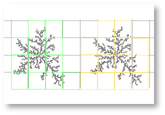
that can affect the actual count. You can see in the image here
that even though the grid calibre and the foreground pixels are
the same on both sides, the number of boxes needed to cover all
of the foreground pixels (and therefore also the distribution
of pixels counted) depends on where the grid is positioned.
Because of this dependence on
the sampling grid's orientation,
FracLac uses
multiple orientations
of the same set of grid calibres to sample an image and delivers
fractal dimensions based on
different methods
of transforming the data from multiple positions.
Sliding Scans
In addition to the "fixed grid" box counting we have discussed here so far, FracLac does "sliding box" scanning to calculate an image feature called sliding box lacunarity (which you might see as Sλ, SΛ, Slacunarity, SLAC, or Slac, all referring to variations of the one type of lacunarity).
The essential feature of a sliding scan is that
one box moves over the image, overlapping itself at each slide.
Thus, compared to a fixed scan, a sliding scan is considerably slower.
The two animations below illustrate how a fixed scan can cover an
entire image with multiple grid sizes before a sliding scan is
done with even one box size.
A couple of pictures say a couple of thousand words.

The figure below illustrates how all that sliding would look if
we drew the box at each location and left it there. In the figure,
the same box was laid over the image for the sliding scan
(top of the figure) and the fixed scan (bottom), and traced for
each location, to highlight the overlap in a sliding scan and the
lack of it in the fixed. When considering this notion,
it is important to note that the distances slid horizontally and
vertically are
options the user sets in FracLac.
There is, accordingly, a notable difference in sampling between fixed and sliding scans. In the regular fixed scan, each part of the image is sampled only once by any particular box size in a series of grid calibres, but in the sliding scan, parts of the image can be resampled multiple times by one box size.
When many calibres of grids are used, the difference in sampling
becomes even more meaningful. To delve into this concept, look at
the image shown here of a scaled version of an 8-segment quadric
fractal (DF=1.50) along with a part of it zoomed in.
The zoomed part is there so you can see the detail as we look at
how sampling is different between fixed and sliding scans using
a series of grid sizes.
Below are pairs of grid images made from the original. The left side of each pair is made from a sliding scan and the right from a fixed scan of the orginal image. The boxes that contained foreground pixels for each type of scan at the same grid calibre are drawn in cyan on each image in the pair. If you hover your mouse over the different items in the list below the pairs, you will see how both grid calibre and scan type affect the number of boxes. Two of the images show the part corresponding to the zoomed in part above, to illustrate the difference in greater detail.
- Grid Calibre = 2 pixels over part of the image
- Grid Calibre = 4 pixels over the same part of the image
- Grid Calibre = 26 pixels over the entire image. At this large calibre, the boxes in the sliding scan overlap so much that they obscure the pattern, whereas it is easy to see in the fixed scan. Note that if the distances to slide horizontally and vertically had been set equal to the box size, then the results for that box size would be essentially a fixed scan.
Re-sampling part of an image in sliding scans dramatically increases the time to scan. It also affects the data gathered, especially as box size increases. Accordingly, rather than the number of boxes, the average pixels per box is used in the calculations from overlapping scans.
tutorial on how to generate
grid images in FracLac.
Lacunarity tutorial
Sliding Box Lacunarity Scan Settings
Local Connected Set
 Another variation in box counting
with FracLac is in sampling for the
local connected fractal dimension (LCFD).
FracLac calculates the LCFD using a technique applied only to
binary images, whereby they
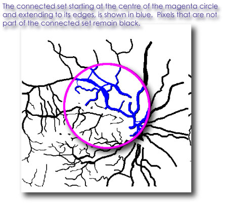
are sampled pixel by pixel in terms of the local connected
set around each pixel, an example of which is shown in the image below.
Another variation in box counting
with FracLac is in sampling for the
local connected fractal dimension (LCFD).
FracLac calculates the LCFD using a technique applied only to
binary images, whereby they
are sampled pixel by pixel in terms of the local connected
set around each pixel, an example of which is shown in the image below.
The basic rule for finding the local connected set is that all foreground pixels that are in the 8x8 environment of a seed pixel are considered connected, and this basic rule is applied to find the connected set for some predetermined arbitrary distance around that starting pixel (the arbitrary distance is a user setting).
 Then, in turn, the rule for data gathering is based on this
connected set rather than the image at large. The actual data
gathering uses fixed boxes, but not in the same way as for a
standard box count. Rather, as is illustrated in the figure below,
a series of changing box calibres is centred, one by one,
on a starting pixel, and the number of pixels that were in the
connected set is counted for each calibre. Because they are centred
on a pixel, the box sizes in a LCFD scan should be
odd numbers. There is also
an option to use circles
as shown in the figure, which was, by the way, generated as an
optional part of the
LCFD scan. With this method of
sampling, the count of boxes at any size is always 1, so the
mass of pixels rather than the count
of boxes is used in the
regression equation
to determine the LCFD.
Then, in turn, the rule for data gathering is based on this
connected set rather than the image at large. The actual data
gathering uses fixed boxes, but not in the same way as for a
standard box count. Rather, as is illustrated in the figure below,
a series of changing box calibres is centred, one by one,
on a starting pixel, and the number of pixels that were in the
connected set is counted for each calibre. Because they are centred
on a pixel, the box sizes in a LCFD scan should be
odd numbers. There is also
an option to use circles
as shown in the figure, which was, by the way, generated as an
optional part of the
LCFD scan. With this method of
sampling, the count of boxes at any size is always 1, so the
mass of pixels rather than the count
of boxes is used in the
regression equation
to determine the LCFD.
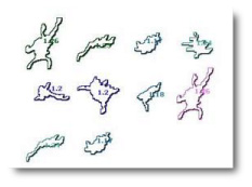
 An important part of LCFD analysis is the potential for visual
presentation (see
Landini).
What you see in the images here is one binary image scanned once,
but
colour-coded multiple times to highlight different types of local
variations as can be applied in diagnostics, for instance, where
"hot spots" need to be detected and located,
with the same area being differentiated for multiple features.
This is discussed further in the
LCFD Analysis page
An important part of LCFD analysis is the potential for visual
presentation (see
Landini).
What you see in the images here is one binary image scanned once,
but
colour-coded multiple times to highlight different types of local
variations as can be applied in diagnostics, for instance, where
"hot spots" need to be detected and located,
with the same area being differentiated for multiple features.
This is discussed further in the
LCFD Analysis page
How to Set up and Interpret a LCFD Scan
How to Calculate the LCFD
Sub Scans and Block Scans
FracLac calculates local DBs for
subareas of an image.
In these cases, the sample is different to start with - rather than
scanning the image as a whole, parts are analyzed individually. But
the actual scanning method is otherwise the same as for regular
fixed grid box counting.
There are two types of sub scans that you can do in FracLac. In the first, portions of an image are automatically selected using ImageJ's particle analyzer. The image above, for instance, shows the results of a single scan of an image containing multiple cells, where each cell was automatically selected, analyzed, and displayed colour-coded according to its calculated DB.

In the second sub scan type, images are divided into blocks. The image blocks are selected systematically or randomly, depending on the user's choices. The image to the right illustrates one type of graphic generated from a rectangular subareas scan. For further discussion, see the glossary and Sub scans page.
FracLac also does block texture analyses for sliding box lacunarity and standard box counts.