Complexity, You Say?
Whatever type of fractal analysis is being done, it always rests on some type of fractal dimension. There are many types of fractal dimension or DF, but all can be condensed into one category - they are meters of complexity. The word "complexity" is part of our everyday lives, of course, but fractal analysts have kidnapped it for their own purposes in fractal analysis. You know the concept already intuitively - you see it with magnification and you ponder it when you discuss image resolution. In fractal analysis, complexity is a change in detail with change in scale.
Scaling rules are at the heart of fractal analysis.
A DF is, in essence, a scaling rule comparing how a pattern's detail changes with the scale at which it is considered - this is what we mean by complexity.
In general, we deduce the scaling rule or fractal dimension, DF, from knowing how something scales. Formally, this idea is about the relationship between N, the number of pieces and ε, the scale used to get the new pieces. We say that: N∝ε-DF
At this point, you may be thinking, "N?? I don't need no stinking N". You may know with great certainty that whenever you have changed the magnification at which you were viewing something, the number of pieces always stayed the same and that only the size changed. But ask yourself this - did the detail change? Detail is what we mean when we say the number of pieces.
Scaling
To understand how all this fits together in the calculations for scaling rules and fractal dimensions, let's look at things differently than everyday life usually asks us to. First consider something you know, patterns such as the familiar Euclidean shapes of elementary geometry. One shape for which scaling is easy to grasp is a simple line. A line, when scaled by, as an example, 1/3, can be seen to be made up of 3 pieces, each 1/3 the length of the original. Nothing cosmic to that. I won't even draw a diagram because it will surely just bore you. But it is kind of interesting to know that it gives us a use for the N in the scaling relationship, and we can figure out that DF = 1.00 in this situation just by substituting into the equation, because 3=(1/3)-1. Maybe you have already expanded this idea and figured out that all this is to say, too, that when scaling a filled square by 1/2, there will always be 4 new pieces, each 1/4 the area of the original, and D would be equal to 2 (e.g., 4=(1/2)-2).
This may seem trivial—that the dimension (or complexity) of a line is 1 and of a filled square 2—but the decidedly untrivial part is that this sort of scaling, the scaling we know and love, is not necessarily the only kind of scaling possible. The Koch fractal line illustrated at the left, for example, scales into 4 new pieces each 1/3 the length of the original.
You can see how it is formed in the animation. Basically, what happens is that the starting piece is scaled down to 1/3 the length it was, then that piece is laid down four times to make a new one that is the length of the original but has more pieces. This goes on forever and the infinite result, alas, we mere mortals cannot see, but is, nonetheless, the Koch fractal pattern.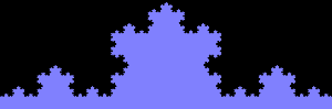 The definitely untrivial point here is that in contrast to the line and square considered above, the scaling rule, DF, for this pattern, even if we could perceive it's infinite nature, is not so obvious—the numbers are 4=(1/3)-DF and this we cannot solve by simple substitution into the scaling rule.
Logs and Limits
How is a Fractal Dimension Calculated?
For the Koch pattern, you have to get out your math assistance device of choice and calculate the DF. I calculate a DF for any case like this by solving the general equation for the scaling rule :N=Aε-DF for its variable, DF, using logs, which shows that the DF is the ratio of the log of the number of new parts N, to the log of scale, ε:DF = log N/log ε.
I stuck an A in there along with N and ε, didn't I? We'll talk later.
You Can Do It
Now that you have all that scaling rule and log stuff down, you can calculate some fractal dimensions.
- For anything scaling like the simple line mentioned above, the number of new parts is equal to the scale-1, and DF = log X/log X = 1.00.
- For the Koch fractal shown earlier, however, DF = log 4/log 3 = 1.26.
- For the 32-segment quadric fractal you surely remember from an earlier page, the pattern scales into 32 new pieces each 1/8 the size of the previous. Therefore, DF = log 32/log 8 = 1.67.
Sometimes You Need a Little Help From Your Friends
The "number of pieces" referred to in the above examples is equivalent to the detail in a pattern, and, for the examples given so far, we needed only to count and measure fairly simple or at least tractable-as-long-as-you-already-know-something-about-them features to find the relationship between scale and detail. But it is not always easy to calculate a DF this way because the relationship between scale and detail is not always readily observable. Just how much would you enjoy counting and measuring to find 32 new parts for every 1/8 scaling in a quadric fractal, for instance? Out of kindness and respect for our tolerance of tedium, therefore, our friends, the fractal analysts, have developed methods to assess the DF indirectly. They have made ways for us to infer the value of complexity from the ratio of changing detail with changing scale (e.g., magnification or resolution in microscopy) approximated by some measure and assigned a number we figure is close enough to its fractal dimension and that is usually a new type of DF. In FracLac, it is the box counting dimension or DB. The basic equation for finding a fractal dimension from such data approximating scale and detail is nearly what we already know from the scaling rule:DF = limε→0[log Nε⁄log ε]where we find the limit as the slope of the regression line for the data. This is a very handy-dandy technique, indeed. Just what we use for N and ε and exactly how this handy technique works for us in box counting with FracLac is explained in the next section.
One other thing to mention is that the fractals discussed here are also called monofractals, to contrast with something else you can analyze with FracLac and which you can read about later, called multifractals.