Another type of analysis FracLac is used for is multifractal analysis. Multifractals are a type of fractal, but they stand in contrast to the monofractals we have discussed so far, in that multifractals scale with multiple scaling rules. 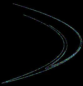
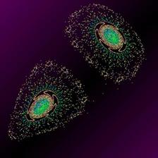
Iterated Henon multifractals generated using the Fractal Growth Models plugin for ImageJ. Click on the images to see them in higher resolution.
As evidenced by the images of Henon multifractals shown here, it is not necessarily easy to determine on inspection whether a pattern is or is not multifractal. So, the question arises, "How do we know if an image is a multifractal?".
To explore multifractal scaling in digital images, you can do a multifractal analysis in FracLac.
What is Multifractal Analysis?. The point of a multifractal analysis is to detect the multi in multifractal scaling. How does multifractal analysis tie in with box counting? It all boils down to the distribution of pixel values in a digital image. That is, to do a multifractal analysis, FracLac uses the box counting grid technique to gather information about the distribution of pixel values (called the "mass distribution"), which becomes the basis for a series of calculations that reveal and explore the multiple scaling rules of multifractals.
You may remember the mass distribution from the discussion of lacunarity on the previous page.
Multifractal Spectra
From the pixel mass distribution, FracLac does calculations and returns data and graphics known as multifractal spectra. Put simply, multifractal spectra are the data or graphs showing how a pattern behaves if amplified in certain ways. To get an intuitive grasp, you might compare the making of multifractal spectra to the experience of zooming in on and distorting parts of an object as you examine it, as in the illustration, which shows a part of a Henon Map magnified and distorted in two different ways.  In a multifractal analysis, the important difference is that it is all done in an orderly fashion, so you can interpret the results with specific rules.
In particular, the rules help us interpret the graphical spectra showing how certain variables behave. Although understanding multifractal analysis requires that you understand the calculations for the variables, it also requires that you understand the graphical element itself. So, whereas the end of this page has a section devoted entirely to calculating the variables that the graphs represent, for now, you need only greet the variables themselves informally, starting with one known as the generalized dimension or D(Q), which is, in essence, one of the distorting lenses of multifractal analysis.
The Generalized Dimension, D(Q)
D(Q) is a distortion of the mean (μ) of the probability distribution for a pattern, and in FracLac, it is a distortion of μ for the distribution of pixel values at some ε from box counting.
What is meant by "a distortion"? To find D(Q), μ is exaggerated by being raised to the arbitrary exponent, Q, then compared again to how the exaggeration varies with ε. Thus, D(Q) basically addresses how mass varies with ε (resolution or box size) in an image, telling how it behaves when you scale or resolve or cut up the image into a series of ε-sized pieces and distort them by Q.(See calculations and Setting Options for Q in a multifractal scan).
Dimensional Ordering
The function, D(Q) vs Q is decreasing, sigmoidal around Q=0, where D(Q=0) ≥ D(Q=1) ≥ D(Q=2) The graphical spectrum D(Q) makes against Q is a marvellous feature of multifractal analysis that, as illustrated in the figure below, can help distinguish types of patterns. The image shows D(Q) spectra from a multifractal analysis of non-, mono-, and multi-fractal images. The non-fractal was a binary contour (a circle) with box counting dimension around 1.0; the fractal, a quadric monofractal Koch Cross with box counting dimension around 1.49, and the multifractal a Henon Map, shown above, with a box counting dimension around 1.29.
One thing in particular to note is that, as the comparison in the figure illustrates, non- and mono-fractals tend to have flatter D(Q) spectra than multifractals. Now, perhaps you have inspected the figure and noticed the similarity between the box counting dimensions and the values at Q=0, and all this has made you wonder if the dimension has been so generalized as to be usefully generally categorized. In fact, one value of the generalized dimension—D(Q=0)—is equal to what we call the "Capacity Dimension", which you can understand as the box counting dimension here. D(Q=1) is equal to what we call the "Information Dimension", and D(Q=2) to the "Correlation Dimension". These three you can make use of when interpreting multifractal analyses, inasmuch as we saw above that there is some natural ordering. We are not going to discuss the generalized dimension further here, except to put this all into perspective and make the point that it helps relate the "multi" in multifractal to the "mono" in monofractal—multifractals have multiple dimensions in the D(Q) vs Q spectra but monofractals are rather flat in that area. Now that really is, marvellous, isn't it?
Other Variables
Some other very important variables are τ, α, and ƒ(α). A typical graph of τ vs Q is illustrated here for the multifractal Henon Map.
 If you have been clicking on the links to the calculations area and studying assiduously, you may have come to know that all of these variables are themselves interrelated. The
image comparing the graphs of D(Q) and α vs Q, for example, illustrates that these two variables hold very similar information.
If you have been clicking on the links to the calculations area and studying assiduously, you may have come to know that all of these variables are themselves interrelated. The
image comparing the graphs of D(Q) and α vs Q, for example, illustrates that these two variables hold very similar information.
It can be enlightening, nonetheless, to consider them separately. Spectra for ƒ(α) vs α, for instance, are illustrated in the image below. As is illustrated in the images, graphs of data from non- and mono-fractal patterns converge on certain values, whereas the spectra from multifractal patterns are typically humped, reflecting the generally observed tendencies in multifractal analyses of these types of patterns. 
Sampling
As was discussed earlier, box counting data depend on
grid position. Because these multifractal spectra are based on pixel distributions determined from box counting, they depend on how the distribution is extracted from an image. Negative Q exponents, for instance, start to be very troublesome, indeed, especially with density distributions that attribute too much importance to very small probabilities that appear in the distribution at some, but not all, grid positions. This is illustrated in the example showing differences in the ƒ(α) vs α spectra at two grid orientations used for sampling the same image with the same set of grid calibres.
What can be done about this sampling issue? One approach to dealing with the problem of pixel distribution being dependent on grid position is to randomly sample a pattern to infer a distribution, which you can do with FracLac's random mass sampling function; but this is subject to several limitations in acquiring an adequate sample.
Another approach is to sample multiple locations fully then select an optimal sample. FracLac's default behaviour for a multifractal analysis is to scan with the grid anchored at each of the four corners of the rectangle enclosing an image, to provide four different spectra similar to what are obtained by rotating the image 90� and reapplying the same series of εs. Then FracLac can select an optimized sample for multifractal analysis based on several criteria (e.g., see the figure below). Another approach is to filter the data using minimum cover or smoothing options. Optimizing and filtering are explained in more detail in the Multifractal Analysis page.
Appendices
Calculations
Variables Used for Multifractal Spectra in FracLac
Please see the Results page for details of the actual methods used to calculate multifractal results.
D(Q)=limε→0[ln I[Q,ε]/ln ε-1]/(1-Q)
I[Q,ε]=N∑ i=1[P(i, ε)]Q
For Q=1, let ε→1, and D(Q)=-lim[N∑ i=1P(i)ln[P(i)]/ln ε]
The probability distribution is found from the number of pixels, M, that were contained in each ith element of a size=ε required to cover an object:
P(i, ε)= M(i, ε)/N∑ i=1M(i, ε)
Thus, P(i) is from the probability distribution of mass for all boxes, i, at this ε
where N∑ i=1P(i, ε)Q=1 = 1
and N∑ i=1P(i, ε)Q=0 = N(ε), the number of boxes containing pixels
P(i, ε)=pixels(i, ε)/N∑ i=1pixels(i, ε)
According to the method of Chhabra and Jensen (Phys. Rev . Lett. 62: 1327, 1989):
μ(I[Q,ε]) = P(i)Q/N∑ i=1P(i)Q
α [Q,ε] = [N∑ i=1(μ (I[Q,ε]])×ln P(i))]/ln ε
ƒ(Q) = [N∑ i=1(μ (I[Q,ε])×ln μ(I[Q,ε]))]/ln ε
τ(Q)=(Q-1)×D(Q)
and ƒ(α [Q,ε])= Q×α(Q)-τ(Q)
References for Calculations
The method of calculating the multifractal spectrum:
A. Chhabra and R.V. Jensen, Direct Determination of the ƒ(α) singularity spectrum, Phys. Rev. Lett. 62: 1327, 1989.
A. N. D. Posadas, D. Giménez, M. Bittelli, C. M. P. Vaz, and M. Flury, Multifractal Characterization of Soil Particle-Size Distributions, Soil Sci. Soc. Am. J.. 65:1361-1367, 2001.