This page is a tutorial/discussion on fractal and lacunarity analyses using BPDs with FracLac. The page has judged you and thinks you know how to use FracLac but could do with some discussion of a few nitty gritty details. Should the page be wrong and you need less grit and more background, try the basic FracLac tutorial and general explanations of box counting and lacunarity.
Are you wondering about certain unpronouncable abbreviations in this manual and in your results files? Do the odd combinations of letters "BPDλ", "BPDL", and "BPD" strike fear in your heart? Worry no longer. Help is here. You won't ever find out how to pronounce it, but here you will learn how to use BPD for fractal and lacunarity analyses.
What BPD is.
Despite what I just said above, you actually can pronounce BPD, if you consider saying "binned probability distributions" a reasonable pronunciation. But what is a BPD? The binned probability distribution is a summary of all of the data for pixel mass from a box count. The data have been sorted and poured into their respective bins so you can keep track of them in big, general groups instead of as thousands and thousands and thousands…well, anyway, lots of individual values. What you get when you order the BPD with your FracLac is a separate distribution for each ε.
FRAC and LAC
The binned distribution is used much like the raw data for finding fractal dimensions and lacunarity for an image. The only real difference is that we use statistics from the distribution instead of the raw data. That statement, however, has some important caveats attached. To elaborate, whereas probability distributions are very popular and we see them everywhere trying to convince us to believe in fanciful ideas like "the mean income" of a nation, there is no definitive distribution for any set of data. The sizes of the bins, for instance, define the way the distribution spreads out. In FracLac, the user can manipulate the bins in the options panel for the relevant scan.
Bins are important, but before we can really know how they affect our results, we need to know a bit about those results. The next section walks you through the basic steps of using BPDs in FracLac.
The Practical Stuff

What you see in the image here is a graph of some of the data in the BPD file for a 136 x 141 pixel image. Each curve represents the binned distribution of pixels per box at a particular box size. Now that's a lot of pixel distributions to be messing around with, no? This section tells you how all those curves can be distilled into a number for the fractal dimension and one for lacunarity for the image. It also gives you some pointers and shows you where to find all the data you might need as you analyze away. You will see various calculations - that will help if you need them to write your paper; but you don't need them to use the program. In addition, this page is loaded with messages and links to help with background as required. Hover over items and click on links if you need more info for something.
The Frac
The fractal dimension from BPDs that you are going to learn about here is not the regular FracLac DB, but a type of DF called a mass dimension or BPDDm. For brevity, we can drop the BPD and use "Dm" here. It is a mass dimension because it comes from mass instead of count as your proxy for detail when finding the limit as the slope of the ln-ln plot.
- The mass you use is the mean of the BPD for any ε. Don't be frightened. You don't have to calculate it - FracLac does that. You just need to know about it in case someone asks what the Dm you are feeding them is made of.
-
In the case that someone does ask, tell them all you
did was to add up all the probabilities times their
midpoints from the BPD.
Or if they are someone grand and complicated,
show them the complicated looking equation for the
mean of the
probability distribution at some ε:
BPDμ[ε]=
BinsΣi=1
(m[i,ε]*p[i,ε])
where m is the mass or
midpoint and p the Probability
reported in the
Probabilities and Masses file.
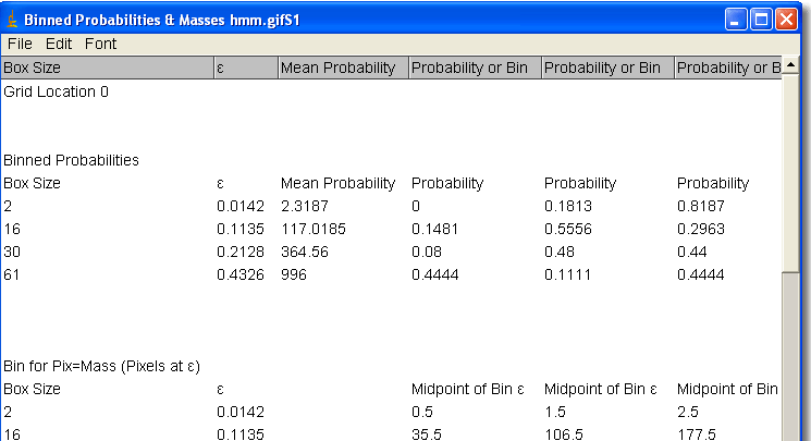
- The basic process is illustrated in the screen shot you should see below of a BPD file generated in FracLac during a standard box count. Hover over the screen shot to illustrate how to find the mean of the BPD at ε for one grid orientation. Note that the distribution and mean are not generated by default. Click here to find out more.
- I really ought to point out that the sample file we are working with has only 4 εs, but I did that on purpose so we could understand it all better. Usually, you have many more sizes, like in the picture you saw above. Now that you know how, if you were faced with all those curves, you would feel so much better having them all boiled down into one number each like we've done for the 4 sizes in the sample file.
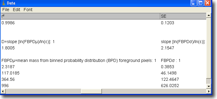
- The next step toward finding the Dm, one number for all box sizes at this orientation, is to find the limit or the ln-ln regression line. You don't have to do that yourself, because FracLac can graph the regression line for you. And you could use all those BPDμε to find the slope for the data set, but you don't have to calculate that yourself, either, of course. It will be waiting for you in the Data File. The Data File complementing the BPD file above is shown in the screen shot below. It appears only if you tell FracLac that you want a Data File instead of or along with your BPD file.
-
To see how these two files are related, hover over the
screenshot to highlight data for the mean in purple on both
the BPD File and the Data File screenshots. You may need to
scroll up or down to get both images on the screen at the
same time. You will also highlight the slope in an orange
box (left and centre) on the Data File.
- The screenshot shows the first column with BPD data for the mean, μ at the first grid orientation; if there had been multiple grid orientations used, there would be several columns of μ for BPD. In that case, to find one value for the entire image, you average all of the Dms over all grid orientations.
- The "F" preceding BPDμ refers to "foreground pixels"
The Lac
BPD lacunarity is a measure of relative variation, essentially the same as the other basic forms of λ that FracLac reports, except, of course, that the data have been sorted prior to calculating. BPDλ is found from the same mean, BPDμε, that the BPDDm is found from, along with the standard deviation, BPDσε, of the BPDε.
- The standard deviation is: BPDσε=√BPDvε, where BPDvε is the variance[ε]
- and the equation for the variance is: BPDv[ε]= BinsΣ i=1 (m[i,ε]−BPDμ[ε]) 2p[i,ε]
- the whole thing, BPDλ for one ε is calculated: BPDλε= ( BinsΣi=1 [m[i, ε]2×p [i,ε]]−BPDμε2 ) ⁄ BPDμε2
- You can find the array of BPDλ in the data file, as we discussed above, along with BPDμ.
You can't stop there, though. Now that you know essential BPDλ, you can take your new knowledge to the Lacunarity Tutorial to learn how to find the various levels of λ including the slope and mean for the whole image. Before you do, however, there is one last point to ponder…
The Bins
The last topic on this page is the number of bins, an option the user sets in different types of scans in FracLac. Earlier, we noted that there is no definitive distribution. What does this mean for the results you get with FracLac? There are two points to be aware of when answering this question. First, it is common practice in statistics to use no less than 5 bins when making frequency distributions. This practical rule translates into FracLac parlance well enough. Too few bins and you get strange results.
Second, it is important to note that
although the number of bins selected does not change with each
ε, the bin midpoints are different for each grid
calibre—that is, FracLac uses a different set of bins
for each ε, rather than one set of bins for the entire
image. FracLac uses 1 as the smallest possible bin size and
determines the maximum based on the user's choice and the
image itself. The actual bin midpoints at each ε
are printed in the data file, as discussed
above. The point of calculating bins
this way is to generate for all εs over an image
relative distributions where the combined results from
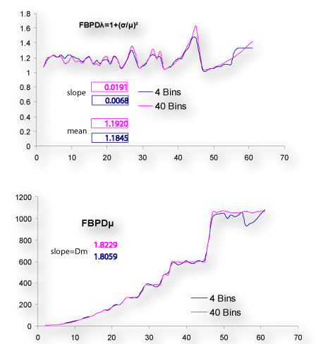
the distributions are robust. The images shown below
illustrate this using 4 bins and 40 bins for the same image.
 .
.
Empties
An important related topic. EBPD and EBPDΛ. This discussion has not touched on the empties BPD, which is another way of looking at an image with box counting. In sum, it accounts for the 2-d space an image occupies a bit differently than does a regular box count. Read the glossary entry to learn more about this result reported with regular box counting.